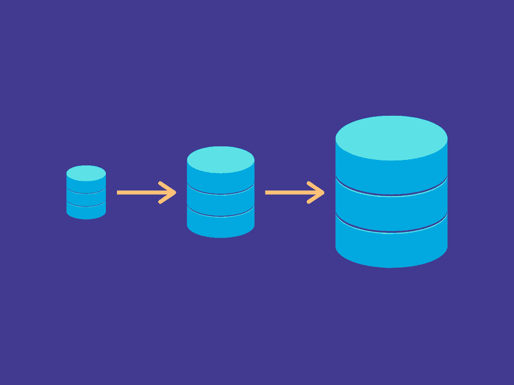
While precise estimates vary, we can all agree on one thing when it comes to data: the amount of it that exists in the world is growing exponentially and will continue to do so.
This means that most data-driven organizations have already experienced the surprising variety of challenges that stem from data scale-up. Fortunately, being prepared for data scalability challenges and staying aware of best practices can help you avoid common issues.
What is data scalability?
The term “scale” is tossed around a lot when we talk about data, often in a frustratingly vague way. That’s because it’s an extremely broad concept that bundles together many factors, each of which can be very complex.
Data scale can encompass any combination of the following:
- The total size of a dataset
- The total number of distinct datasets that you might want to relate to one another
- The frequency at which data is updated
- The frequency at which data is queried
- The relative difficulty of processing queries and/or updates
- The distribution of data usage (ranging from a single machine to globally)
Without diving too deep into the messy details, we can define data scalability as a condition in which you (the human managing the system) don’t have to do anything when any of the above factors change.
Data scalability could also be referred to as “data infrastructure scalability.” These two concepts are intrinsically linked. After all, it is your infrastructure (the various systems you use to collect, store, and transform data) that must actually flex to handle changes in data scale.
A hallmark of data scalability is that you shouldn’t actually notice it happening because your systems should continue to work normally. For example, if the frequency and complexity of queries rise significantly but performance isn’t impacted, your infrastructure is scalable. If performance noticeably suffers to the point where your team isn’t able to work, or you’re not meeting your goals, your data infrastructure is not truly scalable.
Why data scaling is challenging
Historically, performance issues put a hard stop to data scaling before it could reach a noteworthy size. When the only options were older, on-prem processing and storage technologies, there was a limit to how many servers or nodes we could put in place. Some on-prem architectures are more scalable than others; however, there is always a point of diminished performance.
Although “big data” has been a buzzword since the early 2010s, we only recently reached a point where it’s truly attainable, as Matt Turck points out in his recap of the state of data in 2021 (you’ll need to Ctrl-F for “Big Data”). This revolution has been powered by the rise of massively scalable cloud data warehouses.
Even with the virtually unbounded potential of cloud storage, things can still get messy (and expensive) when it comes time to actually put your data to work.
Reducing cost and increasing performance of large-scale data
To save compute resources and reduce costs when scaling your data, your main objective is to prioritize efficiency and eliminate redundancy, while still retaining as much flexibility in your workflow as possible.
How do you actually do that?
Obviously, the answers to that question vary tremendously. But in our conversations with data-driven organizations, we’ve noticed some pain points that appear again and again.
It’s worth noting that Estuary’s focus is in the area of real-time data integration and data operations. So, we specifically investigate pain points in data pipelines and the warehouses they feed into.
However, even if this particular area isn’t your niche, the underlying principles can be applied across your data infrastructure. By targeting these types of issues, you can improve the efficiency of your systems and re-align with your budget.
Pitfall 1 — Expensive queries in OLAP databases
If you store lots of data without planning for its intended use, you’ll eventually run into performance and cost problems. This concept applies to pretty much any type of storage, but we see it the most with OLAP databases.
OLAP (online analytical processing) is a database or data warehouse structure designed to optimize performance in analysis-intensive applications. In contrast to OLTP, which is designed for frequent, small transactions, OLAP aggregates transactions to be less frequent but more complex. Popular cloud data warehouses used for business intelligence, like Snowflake and Bigquery, are OLAP databases.
Though they favor workflows with aggregated, high-throughput transactions, OLAP databases don’t do that on their own. Their actual performance — and by extension, their cost — depends on how you use them.
One common cause of poor performance and ballooning costs in OLAP databases is a pattern of expensive querying.
There are a lot of things that can cause queries to be expensive, but a lot of them boil down to complexity.
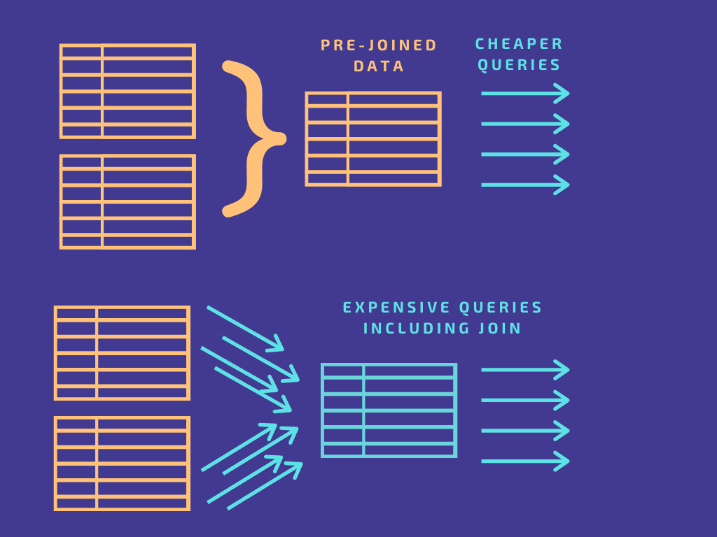
Joining your data can be a great way to begin to broadly simplify your queries. This may seem counter-intuitive because joining doesn’t necessarily reduce data volume; in fact, many types of joins increase data volume. What joining can do is make your queries way cheaper by consolidating one or more steps.
Unless all your data exists in a single table (doubtful), any query you run will invoke one or more joins. By making pre-joined data available in the database, you can skip this step and cut down the cost of each query.
For example, say you’re tracking the performance of an online ad campaign across multiple platforms. Joining the tables on ad ID will save compute power for any query about that ad.
The key is to pre-join data before loading it into storage. In contrast, joining data that’s already in an OLAP database is challenging. Doing so requires you to add several steps to the workflow; namely, adding and querying a materialized view in the database or warehouse (materialized views are actually extremely helpful when used well — more on that later). You’d have to use other tools, like Airflow and dbt, to manage this complex workflow, which adds work as well as latency.
Pre-joining your data is a much more straightforward process. This can be done using an operational transform system such as Spark or Flink, assuming your team includes specialized engineers who work in these systems. When we designed Estuary Flow, we created derivations, a simpler method for powerful stateful joins. They allow any analyst or engineer, regardless of specialty, to pre-join data.
Pitfall 2 — Repeating the same query
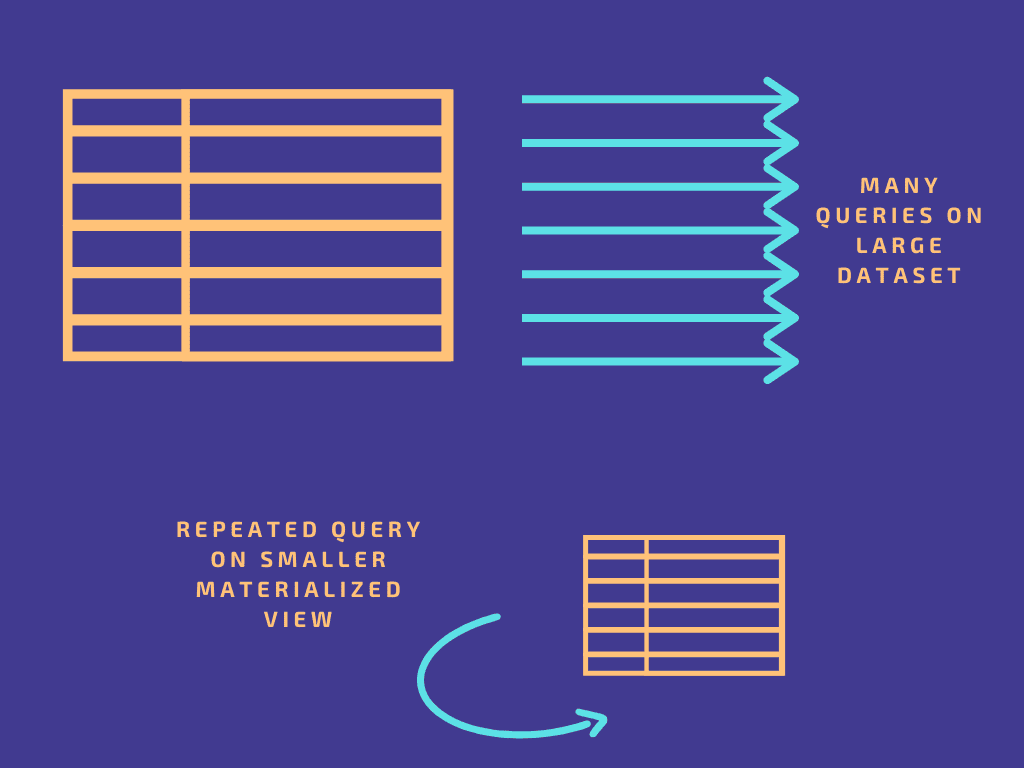
As we’ve already discussed, queries over large datasets cost time, compute resources, money, or a combination. One way to mitigate this is to reduce query complexity; another is to reduce frequency.
It’s common to find that a large percentage of your queries are repeated quite frequently. They’re derived from business questions you need to ask regularly. Questions like:
Which products are selling best right now? How is our ad campaign performing? Have we seen anomalies in recent user behavior?
You may need fresh answers daily, or within minutes or seconds. This is where querying gets really expensive.
Enter the materialized view.
A materialized view is a smaller data object that contains the subset of data resulting from a specific query. Whereas a query happens after data is loaded, a materialized view is a precomputation. The heavy lifting of the computation is done once, and changes to the data are incorporated as they occur, making subsequent updates to the view much cheaper and more efficient than querying the entire database from scratch.
You can create a materialized view directly within the database or data warehouse of your choice. Alternatively, you can use the tool that loads your data, such as Flow, to create the view. This is especially helpful if you want to have the same materialized view in multiple destinations, without managing the manual configuration steps for each warehouse or database.
Flow materializations pull from the cloud-based data pipeline that provides the single source of truth for all your systems. This means that for a given data collection, you can set up two materializations. One uses a query to create a materialized view in your data warehouse; the other perpetuates the full dataset into the warehouse. Both materializations react to new data events within milliseconds, so the materialized view stays in sync with the larger dataset on which it is based.
Pitfall 3 — Rigid pipeline architecture
As you can see, healthy data scaling usually requires some form of transformation to maximize efficiency. Pre-joining and materialized views both fall under this umbrella, as do other types of aggregations and filtering you may use to reduce data volume.
These transformations can occur in different stages of the data lifecycle, so it’s important not to limit where your architecture allows you to perform them. Keep in mind that your method will likely change in the future!
When you’re designing a data pipeline or choosing a vendor to help you, don’t get hung up on the idea of the divide between ETL and ELT. This is a limiting framework, and modern architectures are able to be much more flexible.
For instance, it can be tempting to prioritize flexibility by choosing an ELT model: load all your data into the data warehouse to be transformed on an as-needed basis. By definition, transformations often result in a loss of detail, so you may want to store all data and keep your options open for future queries. However, this large volume of data will diminish performance.
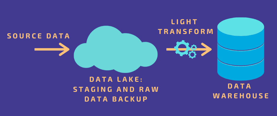
A better solution could be to perform a lighter transformation before loading into the warehouse, where you’ll retain an intermediate level of detail. For example, you might choose to aggregate incoming data in one dimension before storage, and have the potential to perform precise queries in the warehouse later. And if your pipeline uses a data lake as a staging area before uploading to your warehouse, as many do, you can retain the raw data there as a backup in case it’s ever needed.
Of course, the best approach for your organization will vary widely depending on your data structure and your business questions. So, your most important task up front is making sure your engineering team has the ability to change the strategy over time.
Scaling batch and streaming data
The three pitfalls we’ve discussed have a common theme: you can improve your data scalability by applying transformations wisely and allowing yourself the flexibility for future changes.
However, there is one more (major) consideration that you need to account for. So far, this discussion has focused on a batch data paradigm. If you rely on real-time data streaming, scaling can get a lot more complicated.
Essentially, the compute resources that process streaming data must be re-distributed on the fly to match the amount of data flowing through. This means that scaling streaming data is a more complex problem that demands the attention of one or more specialized engineers, or a dedicated streaming solution. If you purchase streaming infrastructure from a vendor, it’s important to make sure that the solution you invest in is built with scaling capabilities.
When we created Flow, we took all of this into account. We addressed the complexity of streaming by creating an automated method to re-distribute resources on the fly based on incoming data volume. At the same time, Flow allows easy, flexible transformations on batch data. Most importantly, the platform enables you to combine both batch and streaming data into a unified pipeline that you can re-arrange, flex, and scale as your use-case inevitably evolves.
Have data scalability challenges that weren’t discussed here? Talk to us on Slack.

